Predicting End-of-Season OBP after Mar/Apr

Introduction / Objective

The goal of this project is to predict a Major League Baseball (MLB) hitter’s end-of-season On-Base Percentage (OBP) based on early season results, specifically after the first two months of the season. This information could be useful to MLB team’s in a variety of ways including assessing player performance, progress, and value in order to make decisions about rosters, potential trades, pickups, lineup options, etc.

This project was originally completed as part of my Advanced Sports Analytics class and has been adapted for this post.

Data

The data for this project was sourced from two datasets:

A dataset provided by our instructor which includes statistics of MLB hitters from March and April of the 2019 season.
Batting statistics from the 2015-2018 seasons sourced from FanGraphs using the baseballr R package.

Though a variety of stats were included in the dataset and explored, the primary statistics utilized in the analysis were Walk Percentage (BB%), Batting Average (AVG), Line Drive Percentage (LD%), the ratio of Home Runs to Fly Balls (HR/FB), Strikeout Percentage (K%), Batting Average for Balls In Play (BABIP), and Fly Ball Percentage (FB%).

    
# load historical hitter data
stats_fangraphs <- baseballr::fg_batter_leaders(x = 2015, y = 2018, league = 'all', qual = 200, ind = 1, exc_p = TRUE)
stats_fangraphs_agg <- fg_batter_leaders(x = 2015, y = 2018, qual = 200, ind = 0, exc_p = TRUE)

# load Mar/Apr 2019 batting data
batting_data <- read_csv('/Desktop/batting.csv')

Data Cleaning

A few steps were required to clean and format the dataset prior to the analysis:

Column names were simplified for easier reference in later code.
Values stored in a “XX%” format were converted to numeric variables.
The HR/FB variable was converted to a proportion.

    
# check NA's 
colSums(is.na(batting))

#simplify column names
colnames(batting) <- sub("^MarApr_", "", colnames(batting))
colnames(batting) <- sub('%', '_perc', colnames(batting))

#remove % signs
for (name in colnames(batting)) {
  if (grepl('_perc', name)) { 
          # if '_perc' is in the name, update the values in the column
          batting <- batting %>%
              mutate(!!name := as.numeric(str_replace_all(!!sym(name), '%', '')))
  } 
}

batting <- batting %>%
  mutate(`HR/FB` = as.numeric(str_replace_all(`HR/FB`, '%', '')) / 100)

Exploration and Visualization

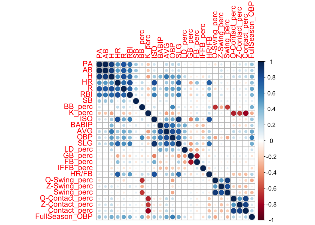
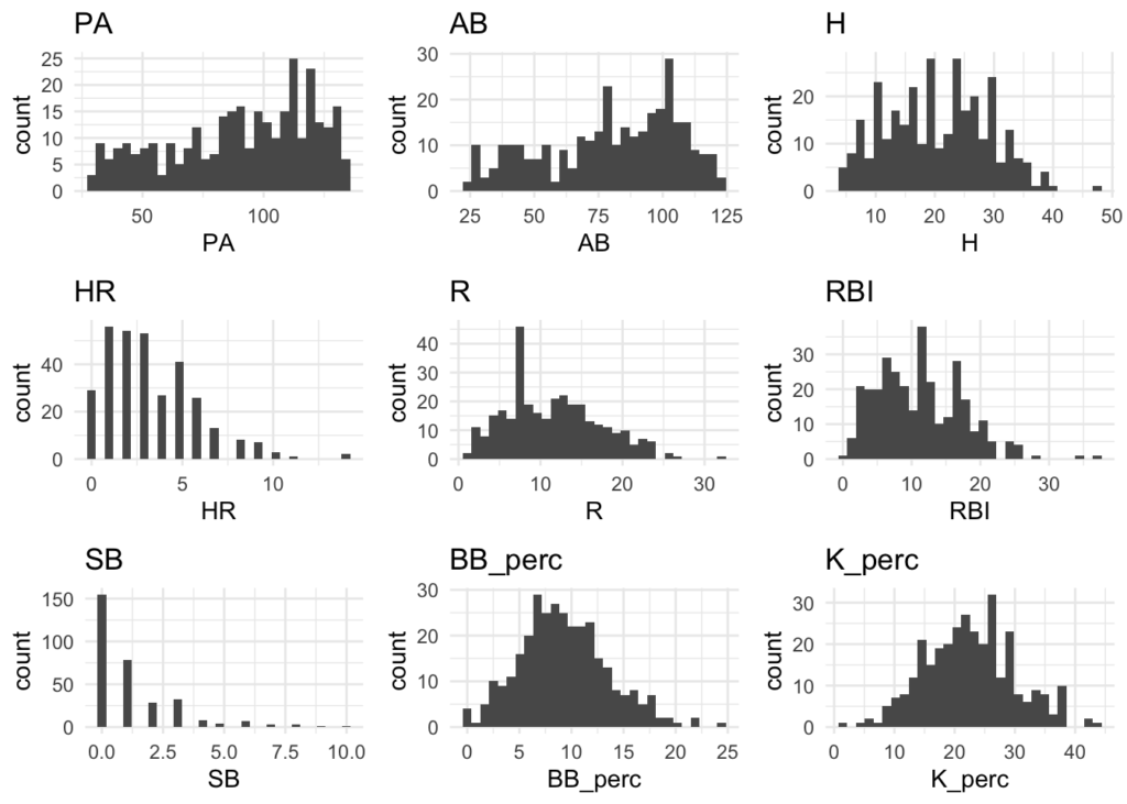
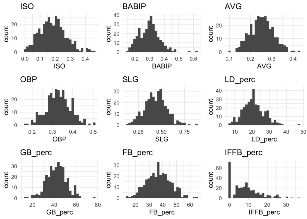
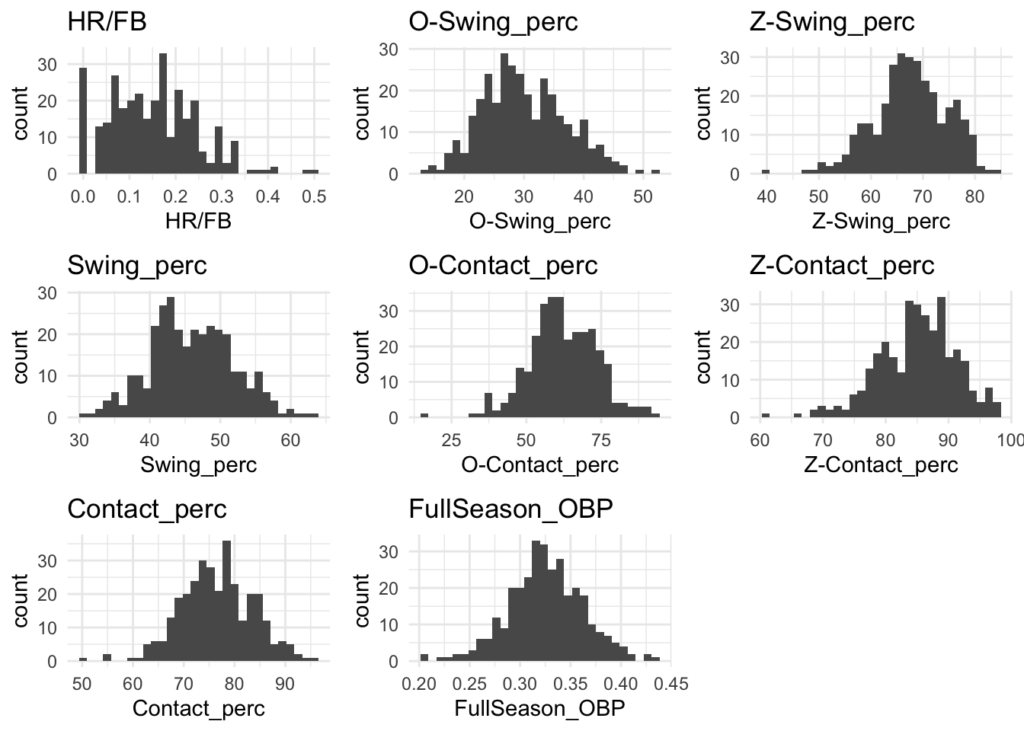
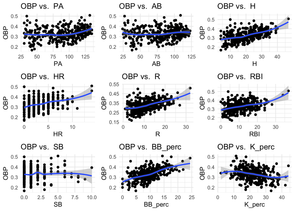
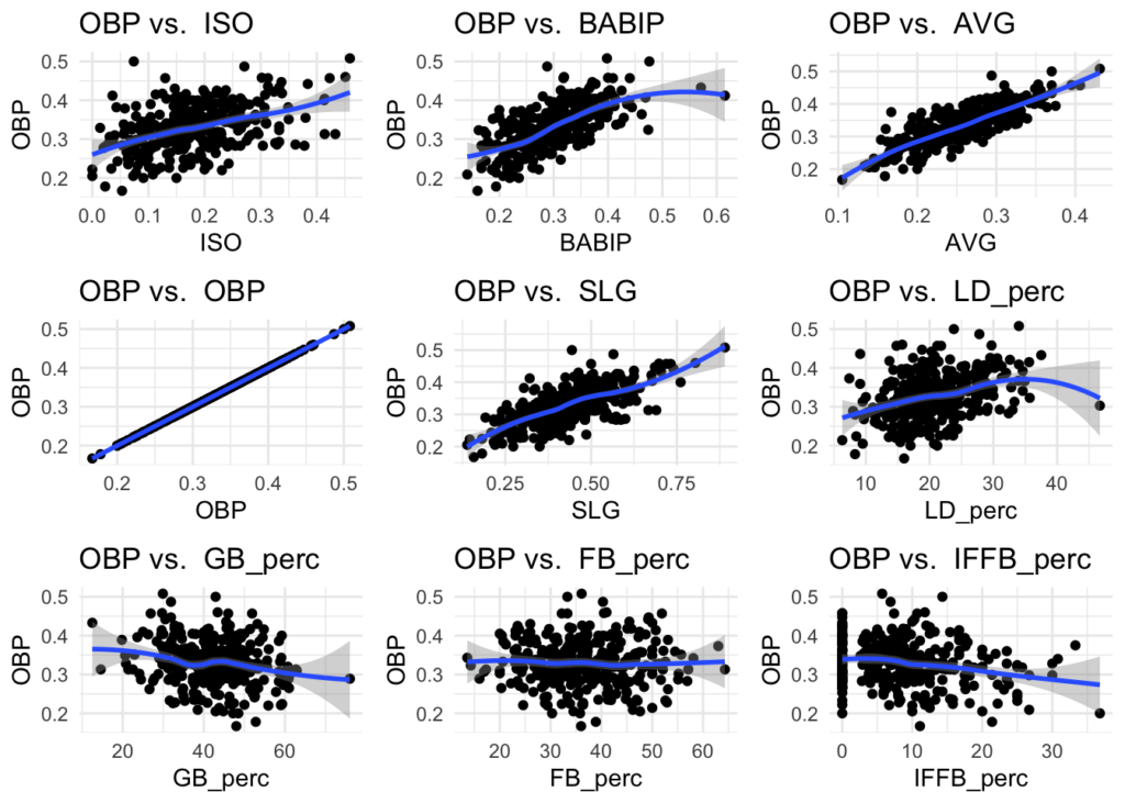
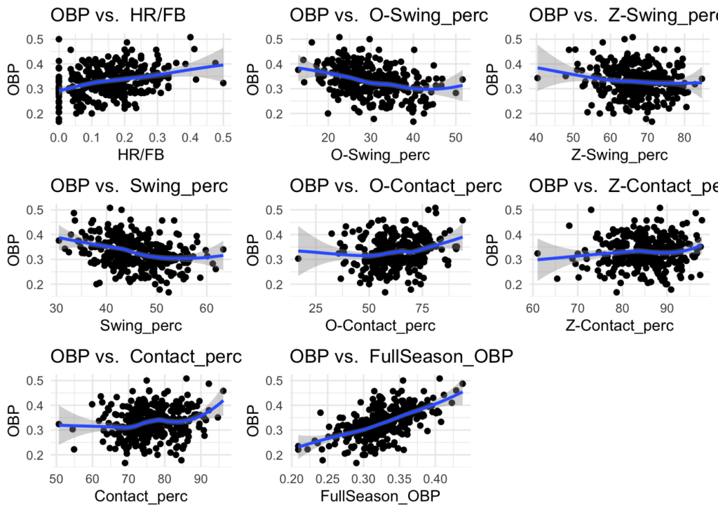
We’ll begin by generating some plots to explore the data and get a feel for some of the important characteristics of the variables/hitting stats we’ll be working with. Specifically, we’ll look for any signs of collinearity between variables, the variables’ distributions, and their relationship with OBP.

Collinearity

There are a number of variables that appear to be collinear with each other. We’ll aim to avoid using these in conjunction when building predictive models.

PA/AB/H/HR/R/RBI
H/AVG/OBP/SLG.
BB% and K% are inversely related to O-Swing% and Contact% respectively.
BABIP/OBS/AVG/SLG
GB_perc/FB_perc are inversely related to each other.

Distributions

Many of the variables appear to be normally distributed. There may be some exceptions like Home Runs (HR) and Stolen Bases (SB), but for the most part this should be good.

Relationship to OBP - QQ Plots

Skimming through these plots, there does appear to be relationships between some of the stats and OBP, such as AVG and SLG. This can give some guidance for what variables to start with when building a model.

    
#calculate + visualize correlations of numeric variables:
cor_df <- batting[, 4:29] %>% na.omit()
correlations <- round(cor(cor_df), 2)
#correlations
corrplot(correlations)


# generate histograms for each variable
plot_list <- list()
names <- colnames(batting[, 4:29])
for (name in names){
  if (is.numeric(batting[[name]])) {
    plot <- batting %>% ggplot(aes(x = .data[[name]])) + 
      geom_histogram() +
      labs(title = name) +
      theme_minimal()
  } else {
    plot <- batting %>% 
      dplyr::select(.data[[name]]) %>% 
      na.omit() %>%
      ggplot(aes(x = .data[[name]])) + 
      geom_bar(stat = "count") +
      labs(title = name) +
      theme_minimal()
  }
  plot_list <- c(plot_list, list(plot))
}

grid.arrange(grobs = plot_list[1:9], ncol = 3)
grid.arrange(grobs = plot_list[10:18], ncol = 3)
grid.arrange(grobs = plot_list[19:27], ncol = 3)


# create qqplots of single variables
plot_list <- list()
for (name in names){
  plot <- batting[, 4:29] %>% 
    ggplot(aes(x = .data[[name]], y = OBP)) +
    geom_point() +
    geom_smooth() +
    labs(title = paste("OBP vs. ", name)) +
    theme_minimal()
  plot_list <- c(plot_list, list(plot))
}

grid.arrange(grobs = plot_list[1:9], ncol = 3)
grid.arrange(grobs = plot_list[10:18], ncol = 3)
grid.arrange(grobs = plot_list[19:27], ncol = 3)

Modeling OBP

Simple Regression / Predictor Selection

We’ll begin with a simple linear regression model to begin to get a sense of what variables correlate well with OBP. This will help inform what predictors we’ll use later on when we employ additional modeling techniques.

We’ll start with the formula below and trim it down based on VIF and Adjusted R-Squared. Since we observed some notable collinearity from our previous exploration, reducing the VIF will be important here.

OBP ~ H + BB% + K% + ISO + BABIP + AVG + SLG + LD% + GB% + FB% + IFFB% + HR/FB + Z-Swing% + Swing% + Contact%

This brings us to two options:

1. 1. OBP ~ BB% + AVG + LD% + HR/FB
  2. OBP ~ BB% + K% + BABIP + FB% + HR/FB

The first set of predictors perform slightly better with a linear model, but since it won’t cost too much, we’ll check both throughout.

    
# collect data into new df for linear model
lm_df <- batting[, 2:28] %>% na.omit()

# define/adjust formulas
form1 <- OBP ~ BB_perc + AVG + LD_perc + `HR/FB`
form2 <- OBP ~ BB_perc + K_perc + BABIP + FB_perc + `HR/FB` 

# check simple linear regression, summary, and vif
fit_lm <- function(data, formula){
  lm_model <- lm(formula, data)
  lm_summary <- summary(lm_model)
  vif_values <- vif(lm_model)
  return(list(summary = lm_summary, vif = vif_values))
}
model1 <- fit_lm(lm_df, form1)
model1$summary
model1$vif
model2 <- fit_lm(lm_df, form2)
model2$summary

Option 1:

	Min	1Q	Median	3Q	Max
Values	-0.019549	-0.007916	-0.001846	0.005723	0.044131

	Estimate	Std. Error	t value	Pr(>\|t\|)
(Intercept)	0.0356135	0.0033496	10.632	<2e-16 ***
BB_perc	0.0074491	0.0001480	50.318	<2e-16 ***
AVG	0.8610646	0.0123612	69.659	<2e-16 ***
LD_perc	0.0002346	0.0001073	2.186	0.0296 *
HR/FB	0.0139324	0.0067911	2.052	0.0410 *
				_

	Value
Residual Standard Error	0.01096 on 315 DF
Multiple R-squared	0.9661
Adjusted R-squared	0.9657
F-statistic	2247 on 4 and 315 DF
p-value	< 2.2e-16

	BB_perc	AVG	LD_perc	`HR/FB`
VIF	1.051944	1.207986	1.150687	1.116361

Option 2:

	Min	1Q	Median	3Q	Max
Values	-0.054625	-0.007276	-0.000794	0.005360	0.045671

	Estimate	Std. Error	t value	Pr(>\|t\|)
(Intercept)	1.122e-01	5.122e-03	21.906	<2e-16 ***
BB_perc	6.615e-03	1.698e-04	38.969	<2e-16 ***
K_perc	-3.475e-03	9.741e-05	-35.674	<2e-16 ***
BABIP	6.078e-01	1.044e-02	58.200	<2e-16 ***
FB_perc	7.548e-04	8.183e-05	9.224	<2e-16 ***
`HR/FB`	1.670e-01	7.659e-03	21.800	<2e-16 ***

	Value
Residual Standard Error	0.01254 on 314 DF
Multiple R-squared	0.9558
Adjusted R-squared	0.9551
F-statistic	1359 on 5 and 314 DF
p-value	< 2.2e-16

	BB_perc	K_perc	BABIP	FB_perc	`HR/FB`
VIF	1.057566	1.070236	1.086499	1.093337	1.085459

Train Models to Predict OBP

We’ll train four different models:

Standard Multiple Linear Regression – Our simple regression from above yielded a fairly high adjusted r-squared of about 0.96, and linear models are highly interpretable, so it should be useful. We’ll use this with both sets of predictors above.
Random Forests – These models are generally pretty versatile, flexible enough to effectively capture non-linear relationships, and are relatively resilient to the effects of outliers, so they seem like they would likely be a good option here. We’ll use this with both sets of predictors above.
Ridge Regression – Since ridge regression builds in some level of feature engineering, we’ll use all of the variables when building this model in case this captures something major that we missed from our simple regression analysis above.
Gradient Boosting – We’ll use this with both sets of predictors from above.

The batter data from March/April 2019 will be split into a training set (75%) and a test set (25%) and we’ll use ten-fold cross validation to fit the models on the training data.

    
# select data for models
reg_df <- batting[, 4:29]

# split data into train/test
set.seed(123) 
train <- reg_df[sample(nrow(reg_df), round(0.75 * nrow(reg_df))) ,] 
test <- reg_df[setdiff(seq_len(nrow(reg_df)), rownames(train)), ]


# set cv protocol
control <- trainControl(method = "repeatedcv", #repeated cv for better accuracy metrics
                        number = 10,
                        repeats = 3,
                        savePredictions = TRUE)

# Train a linear regression model
fit_lm1 <- train(form1,
                method = "lm", data = train,
                trControl = control)

fit_lm2 <- train(form2,
                method = "lm", data = train,
                trControl = control)

# Train a random forest model
fit_rf1 <- train(form1,
                method = "rf", data = train,
                trControl = control)
fit_rf2 <- train(form2,
                method = "rf", data = train,
                trControl = control)

# Train a ridge model
fit_ridge <- train(OBP~H + BB_perc + K_perc + ISO + BABIP + AVG + SLG + LD_perc + GB_perc + FB_perc + IFFB_perc + `HR/FB` + `Z-Swing_perc` + Swing_perc + Contact_perc, 
                   method = 'ridge', data = train, 
                   trControl = control, 
                   preProcess = c("center", "scale"),
                   tuneGrid = expand.grid(lambda = seq(0, 1, by = 0.1)))

# Train a gbm
fit_gbm1 <- train(form1,
                method = "gbm", data = train,
                trControl = control)
fit_gbm2 <- train(form2,
                method = "gbm", data = train,
                trControl = control)

Evaluating the Models

Metrics: We’ll use Mean Average Error (MAE), Root Mean Squared Error (RMSE), and Adjusted R-Squared (Adj. R-Sq) as metrics to evaluate our models.

Results: All four models performed well, but the random forest on the first set of predictors (fit_rf1) performed best on all metrics (MAE, RMSE, Adj. R-Sq). The MAE of about 0.006 suggests that it can estimate a player’s OBP within 6 points on average, which is pretty good.

However, it is important to note that so far, we’ve only demonstrated we can predict current OBP based on current stats. This isn’t exactly the same as predicting end-of-season OBP. To make predictions about the end of the season, we’ll have to make approximations of our predictors to apply the model too. This will likely reduce the accuracy of the final model, so we’ll have to evaluate further.

Test Metrics on All Models (Train & Test Sets):

model	train/test	mae	rmse	rsq
gbm1	test	0.00880	0.0117	0.888
gbm1	train	0.00797	0.0106	0.971
gbm2	test	0.00960	0.0125	0.875
gbm2	train	0.00830	0.0111	0.968
lm1	test	0.00814	0.0117	0.890
lm1	train	0.00797	0.0104	0.971
lm2	test	0.0102	0.0133	0.860
lm2	train	0.00884	0.0124	0.960
rf1	test	0.00644	0.00932	0.933
rf1	train	0.00519	0.00711	0.988
rf2	test	0.00887	0.0114	0.926
rf2	train	0.00715	0.00964	0.983
ridge	test	0.00848	0.0114	0.895
ridge	train	0.00757	0.00988	0.974

    
# Function to compute metrics
compute_metrics <- function(model, data, model_name) {
  # Add predictions to data frame
  data <- data %>%
    mutate(prediction = predict(model, data))

  # Compute metrics and add model name
  metrics(data, truth = OBP, estimate = prediction) %>%
    mutate(model = model_name)
}

# Compute metrics for all models
models <- list(fit_lm1, fit_lm1, fit_rf1, fit_rf2, fit_ridge, fit_gbm1, fit_gbm2)
model_names <- c("lm1 train", "lm2 train", "rf1 train", "rf2 train", 
                 'ridge train', 'gmb1 train', 'gmb2 train')

metrics_df <- purrr::map2_df(models, model_names, compute_metrics, data = train)

# View the results
metrics_df

# add predictions of model back into training set
train$`Linear regression1` <- predict(fit_lm1, train)
train$`Linear regression2` <- predict(fit_lm2, train)
train$`Random forest1` <- predict(fit_rf1, train)
train$`Random forest2` <- predict(fit_rf2, train)
train$`Ridge` <- predict(fit_ridge, train)
train$`Gradient Boost1` <- predict(fit_gbm1, train)
train$`Gradient Boost2` <- predict(fit_gbm2, train)

# Evaluate the performance on training set
train_metrics <- bind_rows(
  metrics(train, truth = OBP, estimate = `Linear regression1`) %>% mutate(model="lm1 train"),
  metrics(train, truth = OBP, estimate = `Linear regression2`) %>% mutate(model="lm2 train"),
  metrics(train, truth = OBP, estimate = `Random forest1`) %>% mutate(model = "rf1 train"),
  metrics(train, truth = OBP, estimate = `Random forest2`) %>% mutate(model = "rf2 train"),
  metrics(train, truth = OBP, estimate = `Ridge`) %>% mutate(model = 'ridge train'),
  metrics(train, truth = OBP, estimate = `Gradient Boost1`) %>% mutate(model = 'gbm1 train'),
  metrics(train, truth = OBP, estimate = `Gradient Boost2`) %>% mutate(model = 'gbm2 train')
)

# Create the new columns
test$`Linear regression1` <- predict(fit_lm1, test)
test$`Linear regression2` <- predict(fit_lm2, test)
test$`Random forest1` <- predict(fit_rf1, test)
test$`Random forest2` <- predict(fit_rf2, test)
test$`Ridge` <- predict(fit_ridge, test)
test$`Gradient Boost1` <- predict(fit_gbm1, test)
test$`Gradient Boost2` <- predict(fit_gbm2, test)


# Evaluate the performance on test set
test_metrics <- bind_rows(
  metrics(test, truth = OBP, estimate = `Linear regression1`) %>% mutate(model = "lm1 test"),
  metrics(test, truth = OBP, estimate = `Linear regression2`) %>% mutate(model = "lm2 test"),
  metrics(test, truth = OBP, estimate = `Random forest1`) %>% mutate(model = "rf1 test"),
  metrics(test, truth = OBP, estimate = `Random forest2`) %>% mutate(model = "rf2 test"),
  metrics(test, truth = OBP, estimate = `Ridge`) %>% mutate(model = 'ridge test'),
  metrics(test, truth = OBP, estimate = `Gradient Boost1`) %>% mutate(model = 'gbm1 test'), 
  metrics(test, truth = OBP, estimate = `Gradient Boost2`) %>% mutate(model = 'gbm2 test')
)

train_metrics

# Combine and format the results
result_df <- bind_rows(train_metrics, test_metrics) %>%
  dplyr::select(-.estimator) %>%
  arrange(.metric, model) %>%
  spread(.metric, .estimate)

result_df

Predicting End-of-Season

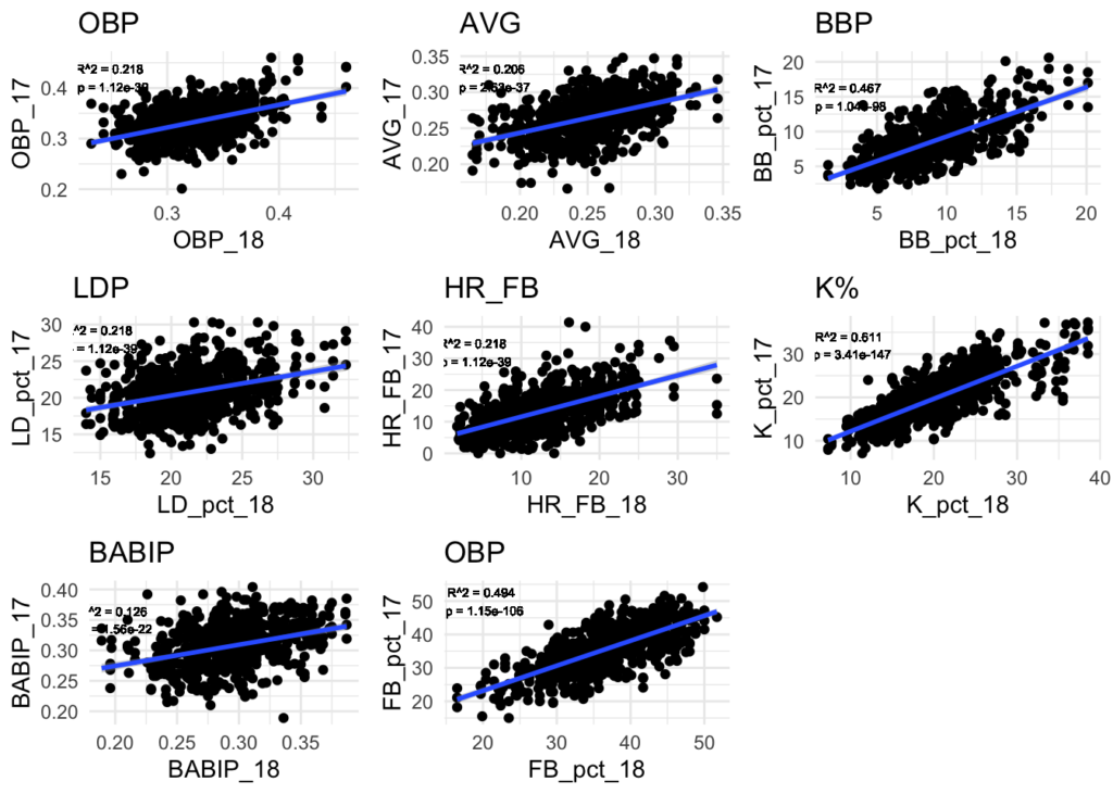
In order to make end-of-season predictions, we’ll assume some amount of regression to the mean for each of the predictors (and possibly overall OBP too). However, instead of just using the league mean of each stat to determine what to regress to, we’ll also take into account the player’s performance historically. To get a sense of how much a player’s historical performance influences their current performance, we’ll compare 2015-2017 stats to 2018 stats for each of the predictors (and OBP). Using a simple linear regression for each predictor, we’ll use the r-squared value as a rough proportion of how much we should factor in the player’s historical performance relative to the overall league mean. Predictors with higher r-squared values mean that past performance correlates better with future performance in that stat. Using the r-squared for the weighting will allow us to give more weight to past performance for such predictors.

Determine Proportion of 2018 Variance explained by 2015-17

Linear Regression of Predictor Variables

This analysis yields the following R-Squared values for each of the variables, and by extension, the proportion or weighting that we’ll use for each to factor in the historical statistics.

Predictor	R-Squared
OBP	0.22
AVG	0.21
BB%	0.47
LD%	0.22
HR/FB	0.22
K_perc	0.61
BABIP	0.13
FB_perc	0.49

    
# prep historical data for analysis
historical_data <- as.data.frame(stats_fangraphs) %>% 
  dplyr::select(playerid, Season, Name, OBP, PA, AVG, BB_pct, LD_pct, HR_FB, K_pct, BABIP, FB_pct)
hist17 <- historical_data %>% filter(Season <= 2017) 
hist18 <- historical_data %>% filter(Season == 2018)

colnames(hist18)[3:12] <- paste0(colnames(hist18)[3:12], "_18")
colnames(hist17)[3:12] <- paste0(colnames(hist17)[3:12], "_17")
historical_data <- merge(hist17, hist18, by = "playerid", all = TRUE) %>% na.omit()

# run linear regressions on 2018~2015 stats for each variable
lm_obp <- lm(OBP_18 ~ OBP_17, historical_data)
lm_avg <- lm(AVG_18 ~ AVG_17, historical_data)
lm_bbp <- lm(BB_pct_18 ~ BB_pct_17, historical_data)
lm_ldp <- lm(LD_pct_18 ~ LD_pct_17, historical_data)
lm_hrfb <- lm(HR_FB_18 ~ HR_FB_17, historical_data)
lm_kp <- lm(K_pct_18 ~ K_pct_17, historical_data)
lm_babip <- lm(BABIP_18 ~ BABIP_17, historical_data)
lm_fbp <- lm(FB_pct_18 ~ FB_pct_17, historical_data)

# plot the graphs with r^2 and p values displayed
plot_obp <- historical_data %>% 
  ggplot(aes(x = OBP_18, y = OBP_17)) + 
  geom_point() + 
  geom_smooth(method = 'lm') + 
  labs(title = 'OBP') +
  geom_text(x = .25, y = .42, size = 2,
            label = paste("R^2 =", format(summary(lm_obp)$r.squared, digits = 3), "\n",
                          "p =", format(summary(lm_obp)$coefficients[2, 4], digits = 3))) + 
  theme_minimal()

plot_avg <- historical_data %>% 
  ggplot(aes(x = AVG_18, y = AVG_17)) + 
  geom_point() + 
  geom_smooth(method = 'lm') + 
  labs(title = 'AVG') +
  geom_text(x = .18, y = .32, size = 2,
            label = paste("R^2 =", format(summary(lm_avg)$r.squared, digits = 3), "\n",
                          "p =", format(summary(lm_avg)$coefficients[2, 4], digits = 3))) +
  theme_minimal()


plot_bbp <- historical_data %>% 
  ggplot(aes(x = BB_pct_18, y = BB_pct_17)) + 
  geom_point() + 
  geom_smooth(method = 'lm') + 
  labs(title = 'BBP') +
  geom_text(x = 3, y = 15, size = 2,
            label = paste("R^2 =", format(summary(lm_bbp)$r.squared, digits = 3), "\n",
                          "p =", format(summary(lm_bbp)$coefficients[2, 4], digits = 3))) +
  theme_minimal()


plot_LDP <- historical_data %>% 
  ggplot(aes(x = LD_pct_18, y = LD_pct_17)) + 
  geom_point() + 
  geom_smooth(method = 'lm') + 
  labs(title = 'LDP') +
  geom_text(x = 15, y = 28, size = 2,
            label = paste("R^2 =", format(summary(lm_obp)$r.squared, digits = 3), "\n",
                          "p =", format(summary(lm_obp)$coefficients[2, 4], digits = 3))) +
  theme_minimal()


plot_hrfb <- historical_data %>% 
  ggplot(aes(x = HR_FB_18, y = HR_FB_17)) + 
  geom_point() + 
  geom_smooth(method = 'lm') + 
  labs(title = 'HR_FB') +
  geom_text(x = 4, y = 32, size = 2, 
            label = paste("R^2 =", format(summary(lm_obp)$r.squared, digits = 3), "\n",
                          "p =", format(summary(lm_obp)$coefficients[2, 4], digits = 3))) +
  theme_minimal()

plot_kp <- historical_data %>% 
  ggplot(aes(x = K_pct_18, y = K_pct_17)) + 
  geom_point() + 
  geom_smooth(method = 'lm') + 
  labs(title = 'K%') +
  geom_text(x = 10, y = 32, size = 2,
            label = paste("R^2 =", format(summary(lm_kp)$r.squared, digits = 3), "\n",
                          "p =", format(summary(lm_kp)$coefficients[2, 4], digits = 3))) + 
  theme_minimal()

plot_babip <- historical_data %>% 
  ggplot(aes(x = BABIP_18, y = BABIP_17)) + 
  geom_point() + 
  geom_smooth(method = 'lm') + 
  labs(title = 'BABIP') +
  geom_text(x = .2, y = .35, size = 2,
            label = paste("R^2 =", format(summary(lm_babip)$r.squared, digits = 3), "\n",
                          "p =", format(summary(lm_babip)$coefficients[2, 4], digits = 3))) + 
  theme_minimal()

plot_fbp <- historical_data %>% 
  ggplot(aes(x = FB_pct_18, y = FB_pct_17)) + 
  geom_point() + 
  geom_smooth(method = 'lm') + 
  labs(title = 'OBP') +
  geom_text(x = 20, y = 50, size = 2,
            label = paste("R^2 =", format(summary(lm_fbp)$r.squared, digits = 3), "\n",
                          "p =", format(summary(lm_fbp)$coefficients[2, 4], digits = 3))) + 
  theme_minimal()

grid.arrange(plot_obp, plot_avg, plot_bbp, plot_LDP, plot_hrfb, plot_kp, 
             plot_babip, plot_fbp, ncol = 3)

Determining What To Regress Each Statistic To

Now, we’ll determine what “mean” to regress to by taking a weighted average of the league mean and each individual player’s historical performance in each stat, where the weighting is based on the R-Squared value from the linear models above. The following table includes those values and their corresponding equations.

Predictor	League Average	Weighted Mean to Regress to
OBP	0.3156614	0.28 * OBP + (1-0.28) * 0.3213672
AVG	0.2487154	0.20 * AVG + (1-0.20) * 0.2511231
BB%	8.1192369	0.51 * BB% + (1-0.51) * 8.5211663
LD%	20.7917329	0.29 * LD% + (1-0.29) * 20.8712743
HR/FB	12.0421304	0.29 * HR/FB + (1-0.29) * 12.9485961
K%	22.0227345	0.61 * OBP + (1-0.61) * 22.0227345
BABIP	0.2977250	0.13 * BABIP + (1-0.13) * 0.2977250
FB%	34.7594595	0.49 * FB% + (1-0.49) * 34.7594595

This will give us a “mean” to regress to for each stat that incorporates an “appropriate” proportion of the player’s historical performance. Note that for any players in the 2019 season without historical data, we’ll just use the league mean as a substitute.

    
# determine the league mean's for each stat across both years
historical_data_agg <- as.data.frame(stats_fangraphs_agg)[, c(1:51, 289)] %>% 
  dplyr::select(playerid, Name, OBP, PA, AVG, BB_pct, LD_pct, HR_FB, K_pct, BABIP, FB_pct, )
stats <- c('OBP', 'AVG', 'BB%', 'LD%', 'HR/FB', 'K%', 'BABIP', 'FB%', 'PA')
means <- c(mean(historical_data_agg$OBP), 
           mean(historical_data_agg$AVG),
           mean(historical_data_agg$BB_pct),
           mean(historical_data_agg$LD_pct),
           mean(historical_data_agg$HR_FB), 
           mean(historical_data_agg$K_pct),
           mean(historical_data_agg$BABIP),
           mean(historical_data_agg$FB_pct),
           mean(historical_data_agg$PA)) 
data.frame(stats, means)

# save r^2 proportions to use for weighted average
r_obp <- 1*as.numeric(format(summary(lm_obp)$r.squared, digits = 3))
r_avg <- 1*as.numeric(format(summary(lm_avg)$r.squared, digits = 3))
r_bbp <- 1*as.numeric(format(summary(lm_bbp)$r.squared, digits = 3))
r_ldp <- 1*as.numeric(format(summary(lm_ldp)$r.squared, digits = 3))
r_hrfb <- 1*as.numeric(format(summary(lm_hrfb)$r.squared, digits = 3))
r_kp <- 1*as.numeric(format(summary(lm_kp)$r.squared, digits = 3))
r_babip <- 1*as.numeric(format(summary(lm_babip)$r.squared, digits = 3))
r_fbp <- 1*as.numeric(format(summary(lm_fbp)$r.squared, digits = 3))


# compute weighted averages to regress to
regress_to_data <- historical_data_agg %>%
  mutate(OBP_RT = r_obp * OBP + (1-r_obp) * mean(historical_data_agg$OBP), 
         AVG_RT = r_avg * AVG + (1-r_avg) * mean(historical_data_agg$AVG), 
         BB_pct_RT = r_bbp * BB_pct + (1-r_bbp) * mean(historical_data_agg$BB_pct), 
         LD_pct_RT = r_ldp * LD_pct + (1-r_ldp) * mean(historical_data_agg$LD_pct), 
         HR_FB_RT = r_hrfb * HR_FB + (1-r_hrfb) * mean(historical_data_agg$HR_FB), 
         K_pct_RT = r_hrfb * K_pct + (1-r_kp) * mean(historical_data_agg$K_pct), 
         BABIP_RT = r_hrfb * BABIP + (1-r_babip) * mean(historical_data_agg$BABIP), 
         FB_pct_RT = r_hrfb * FB_pct + (1-r_hrfb) * mean(historical_data_agg$FB_pct)) %>% 
  dplyr::select(playerid, Name, OBP_RT, AVG_RT, BB_pct_RT, LD_pct_RT, HR_FB_RT, K_pct_RT, 
                BABIP_RT, FB_pct_RT)

head(regress_to_data)

Regression to the Weighted-Mean

To regress to the weighted-mean, we’ll take another weighted average factoring in Plate Appearances (PA) as our sample size to determine how much weight to apply to the Mar/Apr 2019 stats vs. the weighted-mean value computed above. To do this, we’ll use the formula

Regressed STAT = Current_STAT * (PA / N) + STAT_RT * (1 – PA / N),

where we’ll determine N empirically to match the regressed stat’s standard deviation and distribution to that of the historical values.

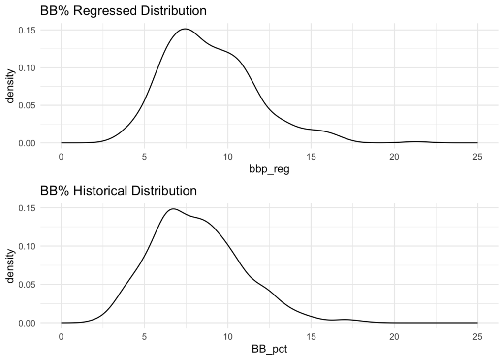
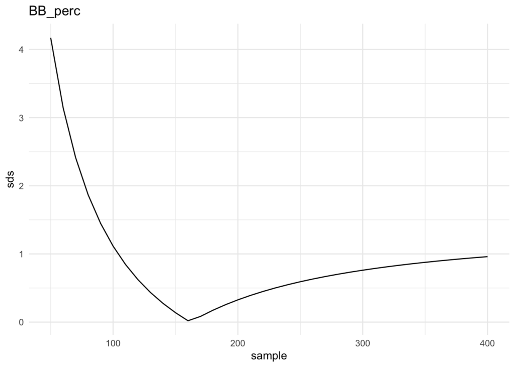
To determine N, we’ll test about a series of values from 50 to 400 and select the one that causes the distribution of the Regressed AVG to have the closest standard deviation to that of the historical data. We’ll also examine the distributions graphically and adjust if necessary so they look similar between the regressed stat and the historical stat. Here are the values that were determined for N for each stat:

Statistic	N
OBP	180
AVG	180
BB%	160
LD%	200
HR/FB	400
K%	130
BABIP	160
FB%	130

Using these values for N gives a distribution that is relatively consistent with the historical distribution for these stats, indicating that it is an appropriate value to use for our weighting.

Code to Determine N

The code for BB% is included as a sample here. The other statistics were determined via the same method. I know I should have written a loop or function to condense the code for the repeated operation across all statistics, but I didn’t, so I won’t copy it all here.

    
# organize data
bat_df <- merge(batting, regress_to_data, by = "playerid", all.x = TRUE) %>%
  dplyr::select(playerid, Name.x, PA, OBP, BB_perc, AVG, LD_perc, `HR/FB`, 
                K_perc, BABIP, FB_perc, FullSeason_OBP, 
                OBP_RT, BB_pct_RT, AVG_RT, LD_pct_RT, HR_FB_RT, K_pct_RT, BABIP_RT, FB_pct_RT) %>%
  mutate(OBP_RT = ifelse(is.na(OBP_RT), mean(historical_data_agg$OBP), OBP_RT), 
         BB_pct_RT = ifelse(is.na(BB_pct_RT), mean(historical_data_agg$BB_pct), BB_pct_RT),
         AVG_RT = ifelse(is.na(AVG_RT), mean(historical_data_agg$AVG), AVG_RT), 
         LD_pct_RT = ifelse(is.na(LD_pct_RT), mean(historical_data_agg$LD_pct), LD_pct_RT),
         HR_FB_RT = ifelse(is.na(HR_FB_RT), mean(historical_data_agg$HR_FB), HR_FB_RT), 
         K_pct_RT = ifelse(is.na(K_pct_RT), mean(historical_data_agg$K_pct), K_pct_RT),
         BABIP_RT = ifelse(is.na(BABIP_RT), mean(historical_data_agg$BABIP), BABIP_RT),
         FB_pct_RT = ifelse(is.na(FB_pct_RT), mean(historical_data_agg$FB_pct), FB_pct_RT))
         
# determine optimal PA weighting for BB_perc
sample <- seq(50, 400, 10)
sds <- numeric()
hist_sd <- sd(historical_data_agg$BB_pct)
for (n in sample) {
  reg <- bat_df$PA / n * bat_df$BB_perc +
         (1 - bat_df$PA / n) * bat_df$BB_pct_RT
  sds <- c(sds, abs(sd(reg) - hist_sd))
}

plot_df <- data.frame(sample, sds)
plot_df %>% ggplot(aes(x = sample, y = sds)) + 
  geom_line() + 
  labs(title = 'BB_perc') +
  theme_minimal()

plot_df %>% filter(sds == min(sds))

# Compute values-to-regress-to based on empircally determined N
bat_df <- bat_df %>%
  mutate(obp_reg = PA / 180 * OBP + (1 - PA / 180) * OBP_RT,
         avg_reg = PA / 170 * AVG + (1 - PA / 170) * AVG_RT, 
         bbp_reg = PA / 160 * BB_perc + (1 - PA / 160) * BB_pct_RT,
         ldp_reg = PA / 200 * LD_perc + (1 - PA / 200) * LD_pct_RT,
         hrfb_reg = PA / 400 * `HR/FB` + (1 - PA / 400) * HR_FB_RT, 
         kp_reg = PA / 110 * K_perc + (1 - PA / 110) * K_pct_RT, 
         babip_reg = PA / 160 * BABIP + (1 - PA / 160) * BABIP_RT, 
         fbp_reg = PA / 120 * FB_perc + (1 - PA / 120) * FB_pct_RT)
         
# plot densities for comparison
dens1 <- bat_df %>% ggplot(aes(x = bbp_reg)) +
  geom_density() +
  labs(title = 'BB% Regressed Distribution') +
  scale_x_continuous(limits = c(0, 25)) +
  theme_minimal()

dens2 <- historical_data_agg %>% ggplot(aes(x = BB_pct)) +
  geom_density() +
  labs(title = 'BB% Historical Distribution') +
  scale_x_continuous(limits = c(0, 25)) +
  theme_minimal()

grid.arrange(dens1, dens2, ncol = 1)

This yields an N of 180 and difference in Standard Deviation (between our distribution and the historical) of 0.01997226.

Combining OBP Model with Regressed Statistics to Predict End-of-Season OBP

Now that we have our regressed statistics for each of the predictors, we can apply the OBP models built above to those in order to estimate the end-of-season OBP.

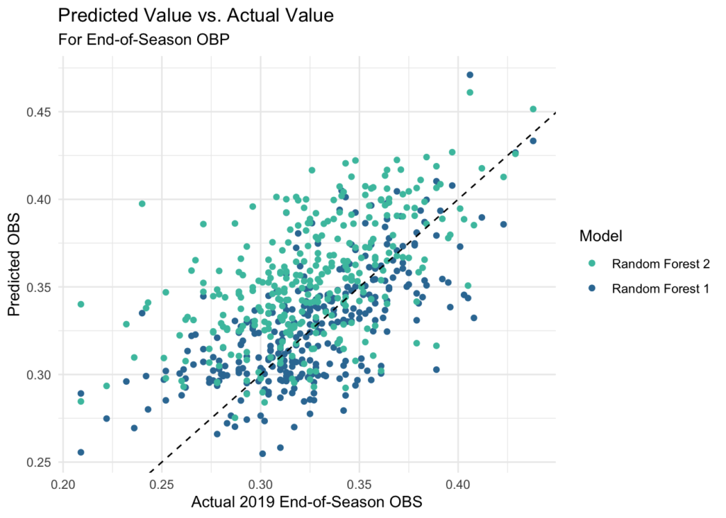
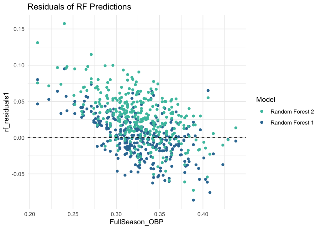
This yields an MAE of about 0.23 for our best performing random forest model. This is ok, but 20 points of OBP is certainly not as good as the 6 we were able to see on the test set of the early season data, so we’re losing a lot as we project toward the end of a season. We can achieve a very modest improvement if we regress this toward the weighted mean for OBP similar to the other statistics, however, this only brings us to about an MAE of 0.22.

    
# organize data so we can predict EOS OBP
eos_df <- merge(batting, bat_df[, c(1, 21:28)], by = "playerid", all.x = TRUE, suffixes = c("", ".x")) %>%
  dplyr::select(-OBP, -AVG, -BB_perc, -LD_perc, -`HR/FB`, -K_perc, -BABIP, -FB_perc)
colnames(eos_df)[colnames(eos_df) == 'obp_reg'] <- 'OBP'
colnames(eos_df)[colnames(eos_df) == 'avg_reg'] <- 'AVG'
colnames(eos_df)[colnames(eos_df) == 'bbp_reg'] <- 'BB_perc'
colnames(eos_df)[colnames(eos_df) == 'ldp_reg'] <- 'LD_perc'
colnames(eos_df)[colnames(eos_df) == 'hrfb_reg'] <- 'HR/FB'
colnames(eos_df)[colnames(eos_df) == 'kp_reg'] <- 'K_perc'
colnames(eos_df)[colnames(eos_df) == 'babip_reg'] <- 'BABIP'
colnames(eos_df)[colnames(eos_df) == 'fbp_reg'] <- 'FB_perc'

# predict EOS OBP using each model
eos_df$eos_obp_lm1 <- predict(fit_lm1, newdata = eos_df)
eos_df$eos_obp_lm2 <- predict(fit_lm2, newdata = eos_df)
eos_df$eos_obp_rf1 <- predict(fit_rf1, newdata = eos_df)
eos_df$eos_obp_rf2 <- predict(fit_rf2, newdata = eos_df)
eos_df$eos_obp_ridge <- predict(fit_ridge, newdata = eos_df)
eos_df$eos_obp_gbm1 <- predict(fit_gbm1, newdata = eos_df)
eos_df$eos_obp_gbm2 <- predict(fit_gbm2, newdata = eos_df)

# plot prediction vs actual value for each model
eos_df %>% ggplot(aes(x = FullSeason_OBP)) + 
  geom_point(aes(y = eos_obp_rf1, color = mako_palette[75])) +
  geom_point(aes(y = eos_obp_rf2, color = mako_palette[50])) +
  geom_abline(slope = 1, intercept = 0, linetype = 'dashed') +
  labs(title = 'Predicted Value vs. Actual Value', 
       subtitle = 'For End-of-Season OBP') +
  scale_y_continuous(name = 'Predicted OBS') +
  scale_x_continuous(name = 'Actual 2019 End-of-Season OBS') +
  scale_color_manual(values = c(mako_palette[75], mako_palette[50]),
                     labels = c("Random Forest 2", "Random Forest 1")) +
  theme_minimal() +
  guides(color = guide_legend(title = "Model")) +
  theme(legend.position = "right") 
  
# residuals plot
eos_df <- eos_df %>% mutate(rf_residuals1 = eos_obp_rf1 - FullSeason_OBP, 
                            rf_residuals2 = eos_obp_rf2 - FullSeason_OBP)
eos_df %>% ggplot(aes(x = FullSeason_OBP)) +
  geom_point(aes(y = rf_residuals1, color = mako_palette[75])) +
  geom_point(aes(y = rf_residuals2, color = mako_palette[50])) +
  geom_hline(yintercept = 0, linetype = 'dashed') +
  scale_color_manual(values = c(mako_palette[75], mako_palette[50]),
                     labels = c("Random Forest 2", "Random Forest 1")) +
  labs(title = 'Residuals of RF Predictions') +
  theme_minimal() +
  guides(color = guide_legend(title = "Model")) +
  theme(legend.position = "right")

# compute MAE, MSE metrics
MAE1 <- mean(abs(eos_df$rf_residuals1))
RMSE1 <- sqrt(mean((eos_df$rf_residuals1)^2))
MAE2 <- mean(abs(eos_df$rf_residuals2))
RMSE2 <- sqrt(mean((eos_df$rf_residuals2)^2))
metrics <- c('MAE1', 'RMSE1', 'MAE2', 'RMSE2')
values <- c(MAE1, RMSE1, MAE2, RMSE2)
data.frame(metrics, values)

# obp_weighted_pred
eos_df$weighted_prediction = eos_df$OBP * .5 + eos_df$eos_obp_rf1 * (1 -.5)

# compute MAE, MSE metrics on weighted prediction
MAE <- mean(abs(eos_df$weighted_residuals))
RMSE <- sqrt(mean((eos_df$weighted_residuals)^2))
metrics <- c('MAE', 'RMSE')
values <- c(MAE, RMSE)
data.frame(metrics, values)

Final Results / Conclusions

With OBP Weighting

Metrics	Values
MAE	0.02251379
RMSE	0.02859316

Without OBP Weighting

Metrics	Values
MAE (Model 1)	0.02300048
RMSE (Model 1)	0.02928569
MAE (Model 2)	0.03557778
RMSE (Model 2)	0.04386678

With a combination of machine learning techniques and regression to the mean, we were able to build a model that projects player’s end-of-season On-Base Percentage based on a selection of batting statistics from the early months (Mar/Apr) of a season. This model can predict with an average error of about .022 (22 pts of OBP). This is an ok result, though I was hoping for a bit higher considering how accurate the initial OBP models looked. However, we can also consider that the model tends to over project players who finished on the lower end of OBP and under project players who finished on the higher end, so depending on the context, it may still prove useful.